Model Specification

Evaluation Geometries

In order to calculate first order corrections with respect to the chosen scattering distributions, the so-called fn-coefficients have to be evaluated. From the general definition of the fn-coefficients (9) it is apparent that they are in principle dependent on \(\theta_0,\phi_0,\theta_{ex}\) and \(\phi_{ex}\). If the series-expansions ((6) and (7)) contain a high number of Legendre-polynomials, the resulting fn-coefficients turn out to be rather lengthy and moreover their evaluation might consume a lot of time. Since usually one is only interested in an evaluation with respect to a specific (a-priori known) geometry of the measurement-setup, the rt1-module incorporates a parameter that allows specifying the geometry at which the results are being evaluated. This results in a considerable speedup for the fn-coefficient generation.

The measurement-geometry for a given RT1 class instance can be set via one of the following options:

• For monostatic measurement geometry, use: RT1.set_monostatic()

• For bistatic measurement geometry, use: RT1.set_bistatic():

To clarify the definitions, the used angles are illustrated in Fig. 3.

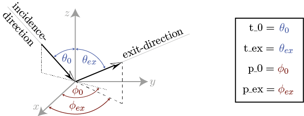
Fig. 3 Illustration of the used incidence- and exit-angles

Monostatic Evaluation

Monostatic evaluation refers to measurements where both the transmitter and the receiver are at the same location. To use monostatic geometry, call RT1.set_monostatic().

In terms of spherical-coordinate description, this is equal to (see Fig. 3):

\[\begin{split}\theta_{ex} &= \theta_0 \\ \phi_{ex} &= \phi_0 + \pi\end{split}\]

Since a monostatic setup drastically simplifies the evaluation of the fn-coefficients, setting the module exclusively to monostatic evaluation results in a considerable speedup.

The module is set to be evaluated at monostatic geometry by setting:

R = RT1(...)
R.set_monostatic(p_0=...)   # use monostatic evaluation geometry with a fixed azimuth angle

R.set_geometry(t_0=...)     # update the angles used for evaluating the model
R.calc(...)                 # calculate the result

Note

• For monostatic geometry, the values of t_ex and p_ex are automatically set to t_ex = t_0 and p_ex = p_0 + pi

• For azimuthally symmetric phase-functions [1], the value of p_0 will have no effect on results for monostatic calculations! In this case, using a fixed value (e.g. p_0=0) will further speed up evaluations!

[1]

This referrs to any phase-function whose generalized scattering angle parameters satisfy a[1] == a[2]. The reason for this simplification stems from the fact that the azimuthal dependency of a generalized scattering angle with a[1] == a[2] can be expressed in terms of \(\cos(\phi_0 - \phi_{ex})^n\). For the monostatic geometry this reduces to \(\cos(\pi)^n = 1\) independent of the choice of \(\phi_0\).

Bistatic Evaluation

Bistatic evaulation refers to measurements where the transmitter and receiver are at different locations. To use bistatic geometry, call RT1.set_bistatic().

Since evaluation of the coefficients required to evaluate bistatic interaction contributions can be demanding, fixing some of the angles can greatly speed up computation times.

To fix an angle, simply pass the value to RT1.set_bistatic().

R = RT1()
R.set_bistatic(t_0=..., p_0=...)   # use bistatic evaluation geometry with fixed source-location

R.set_geometry(t_ex=..., p_ex=...) # update angles used for evaluating the model
R.calc(...)                        # calculate the result

Note

• Whenever a single angle is set fixed, the calculated fn-coefficients are only valid for this specific choice!

Linear combination of scattering distribution functions

Aside of directly specifying the scattering distribution function by choosing one of the implemented rt1_model.volume or rt1_model.surface objects, you can also define parameterized linear-combinations of the distributions to allow consideration of more complex scattering characteristics.

Creating linear combinations of existing distribution functions can be done with the volume.LinComb and surface.LinComb classes which expect a list of weighting-factors and associated distribution functions as input.

The basic usage is as follows:

from rt1 import volume, surface

V = volume.LinComb([(0.5, volume.Isotropic()), (0.5, volume.HenyeyGreenstein(t=0.4, ncoefs=10)])
SRF = surface.LinComb([(0.5, surface.Isotropic()), (0.5, surface.HenyeyGreenstein(t=0.4, ncoefs=10)])

The resulting volume-class element can now be used completely similar to the pre-defined scattering phase-functions.

More details on how to create linear-combinations with the rt1_model package are provided in the Linear combinations of distribution functions example.

Note

Since one can combine functions with different choices for the generalized scattering angle (i.e. the a-parameter), and different numbers of expansion-coefficients (the ncoefs-parameter) LinCombV() will automatically combine the associated Legendre-expansions based on the choices for a and ncoefs.

The attributes .a, .calc_scattering_angle and .ncoefs of the resulting surface/volume object are therefore NOT representative for the generated combined phase-function!

Volume scattering functions

Linear-combinations of volume scattering distribution functions can be used to generate combined volume-scattering functions of the form:

\[\hat{p}_{combined}(\theta_0,\phi_0,\theta_{ex},\phi_{ex}) = \sum_{n=0}^N w_n * \hat{p}_n(\cos(\Theta_{a_n})) = \sum_{n=0}^N w_n * \sum_{k=0}^{K_n} \hat{P}_k(\cos(\Theta_{a_n})) * p^{(n)}_k\]

where \(\hat{p}_n(\cos(\Theta_{a_n}))\) denotes the scattering phase-functions to be combined, \(\cos(\Theta_{a_n})\) denotes the individual scattering angles (8) used to define the scattering phase-functions \(w_n\) denotes the associated weighting-factors, \(p_k^{(n)}\) denotes the \(\textrm{k}^{\textrm{th}}\) Legendre-expansion-coefficient (7) of the \(\textrm{n}^{\textrm{th}}\) phase-function and \(\hat{P}_k(x)\) denotes the \(\textrm{k}^{\textrm{th}}\) Legendre-polynomial.

Note

A volume-scattering phase-function must obey the normalization condition: \(\int_0^{2\pi}\int_0^{\pi} \hat{p}(\theta,\phi,\theta',\phi') \sin(\theta') d\theta' d\phi' = 1\)

If each individual phase-function that is combined already satisfies this condition, the weighting-factors \(w_n\) must equate to 1, i.e.: \(\sum_{n=0}^N w_n = 1\)

Surface scattering functions

Linear-combinations of surface-scattering distribution functions (BRDF’s) can be used to generate combined surface-scattering function of the form:

\[BRDF_{combined}(\theta_0,\phi_0,\theta_{ex},\phi_{ex}) = \sum_{n=0}^N w_n * BRDF_n(\cos(\Theta_{a_n})) = \sum_{n=0}^N w_n * \sum_{k=0}^{K_n} \hat{P}_k(\cos(\Theta_{a_n})) * b^{(n)}_k\]

where \(BRDF_n(\cos(\Theta_{a_n}))\) denotes the BRDF’s to be combined, \(\cos(\Theta_{a_n})\) denotes the individual scattering angles (8) used to define the BRDF’s \(w_n\) denotes the associated weighting-factors, \(b_k^{(n)}\) denotes the \(\textrm{k}^{\textrm{th}}\) Legendre-expansion-coefficient (6) of the \(\textrm{n}^{\textrm{th}}\) BRDF and \(\hat{P}_k(x)\) denotes the \(\textrm{k}^{\textrm{th}}\) Legendre-polynomial.

Note

A BRDF must obey the following normalization condition: \(\int_0^{2\pi}\int_0^{\pi/2} BRDF(\theta,\phi,\theta',\phi') \cos(\theta') \sin(\theta') d\theta' d\phi' = R(\theta_0,\phi_0) \leq 1\) where \(R(\theta_0,\phi_0)\) represents the hemispherical reflectance which must be lower or equal to 1.

In order to provide a simple tool that allows validating the above condition, the function plot.hemreflect() numerically evaluates the hemispherical reflectance using a simple Simpson-rule integration-scheme and generates a plot that displays \(R(\theta_0,\phi_0)\).

Note

If the expansion-coefficients of the BRDF and volume-scattering phase-function exceed a certain number (approx. ncoefs > 20) one might run into numerical precision errors.